Who’s Going to Win the Premiership?
It’s an interesting question isn’t it? With just 6 weeks to go, there are still seven teams that can mathematically win the English League title. I thought it would be an interesting educational exercise in statistics to demonstrate a monte carlo method of predicting probabilities. You can download the spreadsheet I used to see how it all works here. I did do all this in SAS code (geeky statistics software) but most of you won’t have that so Excel will have to do.
“Monte Carlo Method” is the name given to a probability exercise when you want to find out how likely an outcome is when you only have limited information. You assume that inputs will happen in a certain random manner and then you run random simulations a number of times to see how often different outcome happen.
Monte Carlo simulation performs risk analysis by building models of possible results by substituting a range of values—aprobability distribution—for any factor that has inherent uncertainty. It then calculates results over and over, each time using a different set of random values from the probability functions. Depending upon the number of uncertainties and the ranges specified for them, a Monte Carlo simulation could involve thousands or tens of thousands of recalculations before it is complete. Monte Carlo simulation produces distributions of possible outcome values.
By using probability distributions, variables can have different probabilities of different outcomes occurring. Probability distributions are a much more realistic way of describing uncertainty in variables of a risk analysis. Common probability distributions include:
Normal – Or “bell curve.â€Â The user simply defines the mean or expected value and a standard deviation to describe the variation about the mean. Values in the middle near the mean are most likely to occur. It is symmetric and describes many natural phenomena such as people’s heights. Examples of variables described by normal distributions include inflation rates and energy prices.
Lognormal – Values are positively skewed, not symmetric like a normal distribution. It is used to represent values that don’t go below zero but have unlimited positive potential. Examples of variables described by lognormal distributions include real estate property values, stock prices, and oil reserves.
Uniform – All values have an equal chance of occurring, and the user simply defines the minimum and maximum. Examples of variables that could be uniformly distributed include manufacturing costs or future sales revenues for a new product.
Triangular – The user defines the minimum, most likely, and maximum values. Values around the most likely are more likely to occur. Variables that could be described by a triangular distribution include past sales history per unit of time and inventory levels.
PERT- The user defines the minimum, most likely, and maximum values, just like the triangular distribution. Values around the most likely are more likely to occur. However values between the most likely and extremes are more likely to occur than the triangular; that is, the extremes are not as emphasized. An example of the use of a PERT distribution is to describe the duration of a task in a project management model.
Discrete – The user defines specific values that may occur and the likelihood of each. An example might be the results of a lawsuit: 20% chance of positive verdict, 30% change of negative verdict, 40% chance of settlement, and 10% chance of mistrial.
During a Monte Carlo simulation, values are sampled at random from the input probability distributions. Each set of samples is called an iteration, and the resulting outcome from that sample is recorded. Monte Carlo simulation does this hundreds or thousands of times, and the result is a probability distribution of possible outcomes. In this way, Monte Carlo simulation provides a much more comprehensive view of what may happen. It tells you not only what could happen, but how likely it is to happen.
What does all that mean? Well let’s have a look at the Premiership.
We know what the current table is. You can click on any column to sort it by that value.
[table id=2 /]
Now, assume that each team has an equal chance of winning, drawing or losing each of their final games. We can run a thousand random simulations where we see what happens and than examine how many times each team comes top of the table. You’ll find the code for this in sheet “Base Code” and the actual simulation in “Base Run”.
These are the probabilities.
| Liverpool | 48.1% |
| Manchester City | 32.6% |
| Chelsea | 17.9% |
Of course, that’s not realistic. Some teams are better than others and so the idea that they all have an equal chance of winning, losing or drawing each game is a nonsense. What we can do is look at each team’s performance so far this season and calculate how often they won, lost or drew.
| Team | Win | Draw | Lose |
|---|---|---|---|
| Liverpool | 68.75% | 15.625% | 15.625% |
| Chelsea | 65.625% | 18.75% | 15.625% |
| Manchester City | 70% | 13.333% | 16.666% |
| Arsenal | 59.375% | 21.875% | 18.75% |
| Everton | 54.839% | 29.032% | 16.129% |
| Tottenham | 53.125% | 15.625% | 31.25% |
| Manchester United | 50% | 18.75% | 31.25% |
We can see that Manchester City have the greatest probability of winning a game, but Liverpool and Chelsea have the lowest probability of losing.
Let’s feed that back into our model. The code is in “Second Code” and the actual simulated run is in “Second Run”. These are the results we get.
| Manchester City | 52.2% |
| Liverpool | 38.2% |
| Chelsea | 9.4% |
| Arsenal | 0.2% |
That’s quite a bit different isn’t it? What’s really interesting is that Arsenal wins the title in 2 of the 1000 simulations I ran.
We can do other interesting stuff with the simulations. For example, we could see by how many points a winning team won on average, or we could produce a probability table for the final order of teams.
I’m sure you could think of ways to improve the model. For example, some of the games that our top teams are going to play will be against each other, so our model should take that into account (if team A wins then B needs to lose). I’ve also assumed a static goal difference (so sometimes when a team wins the league it’s on goal difference), but we could easily build a model that looks at the average goal difference in a win, lose or draw for each team and adds that on to their goal difference tally depending on the result. Heck, we could even produce a sub-model that looks at how the goal difference is distributed for each team when it wins, loses or draws (i.e. if it wins, is it 50% likely to be +1, 25% likely to be +2 etc) and include that in the calculations.
One last thought. You might be wondering how accurate this kind of thing is and whether it is used in the real world. Well the picture below is a snapshot of the Betfair Exchange market for the Premiership title, as of 10pm on the 30th of March.
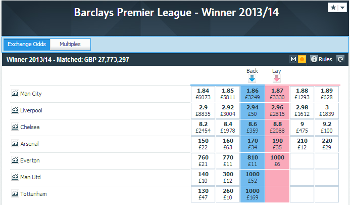
We can take the midpoint between the back and lay prices and calculate an implied probability of winning.
| Team | Peter’s Model | Betfair |
|---|---|---|
| Manchester City | 52.2% | 53.6% |
| Liverpool | 38.2% | 33.9% |
| Chelsea | 9.4% | 11.5% |
| Arsenal | 0.2% | 0.1% |
Not bad huh? My model over predicts Liverpool compared to the betting market, but I suspect ironing out the goal difference component might resolve that.
Who said hard sums were boring?
Update
I’ve updated the model to take into account that Liverpool play both Manchester City and Chelsea. The updated spreadsheet reflects this and can be found in the same place.
| Team | Peter’s Model | Betfair |
|---|---|---|
| Manchester City | 51.4% | 53.6% |
| Liverpool | 35.0% | 33.9% |
| Chelsea | 13.4% | 11.5% |
| Arsenal | 0.2% | 0.1% |
One also needs to figure in the strength of each team’s remaining
opponents. Some have easier final stretches than others. Complicated by
the fact that, as Chelsea were shown on Saturday, at this stage of the
season team battling for its life in or just out of the relegation zone,
like Palace, can be a more difficult opponent than a team around or
just below mid-table who are cruising home to safety with not much left
to play for.
Yes, an even more complicated model could do that (and I have something coded in SAS to that end).
Oh my goodness, my head hurts! But in that way that feels good when you know that the creaking brain cells are given a necessary jolt :)
Although I must confess I have zero interest in football, this has caught my attention as being a poker player, I spend a lot of my time with the monte carlo method, using it to calculate probable hand strengths etc
And as someone who was totally put off by maths for most of his life, one of the great joy of poker has been my discovery of the sublime pleasures of such arcane delights as probabilities,combinatorics and statistics.
Not to mention the fact that it gives me a whole new insight into articles like this one :)